Example2 - Real data set

In this second example we will explore more functionalities with a real dataset from a CLT building, for more info [APTF20].

First of all we import the necessary modules. Then we import the dataset we want to analyse and assign it to a variable. All the files needed to run this example are available here.

   import numpy as np
   from pyoma2.algorithms import FSDD, SSIcov, pLSCF
   from pyoma2.setup import SingleSetup
   from pyoma2.support.utils.sample_data import get_sample_data

   # load example dataset for single setup
   data = np.load(get_sample_data(filename="Palisaden_dataset.npy", folder="palisaden"), allow_pickle=True)

Now we can proceed to instantiate the SingleSetup class, passing the dataset and the sampling frequency as parameters

# create single setup
Pali_ss = SingleSetup(data, fs=100)

If we want to be able to plot the mode shapes, once we have the results, we need to define the geometry of the structure. We have two different method available that offers unique plotting capabilities: * The first method def_geo1() enables users to visualise mode shapes with arrows that represent the placement, direction, and magnitude of displacement for each sensor. * The second method def_geo2() allows for the plotting and animation of mode shapes, with sensors mapped to user defined points.

_geo1 =  get_sample_data(filename="Geo1.xlsx", folder="palisaden")
_geo2 =  get_sample_data(filename="Geo2.xlsx", folder="palisaden")

Pali_ss.def_geo1_by_file(_geo1)
Pali_ss.def_geo2_by_file(_geo2)

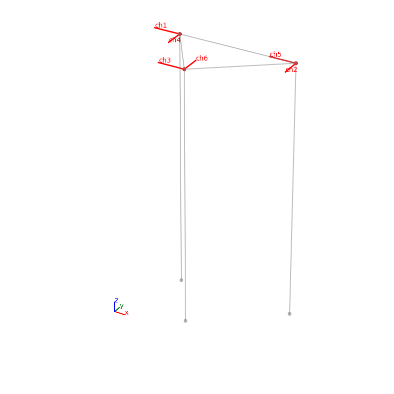
Once we have defined the geometry we can show it calling the plot_geo1() or plot_geo2() methods.

# Plot the geometry (geometry1)
fig, ax = Pali_ss.plot_geo1()
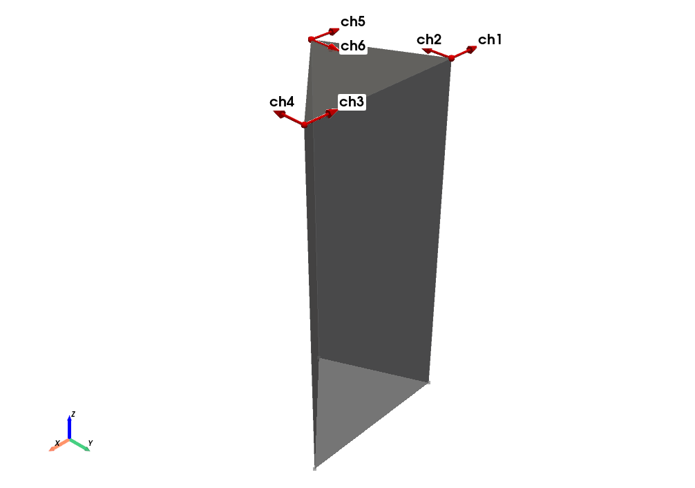
# (geometry2) with pyvista
_ = Pali_ss.plot_geo2(scaleF=2)
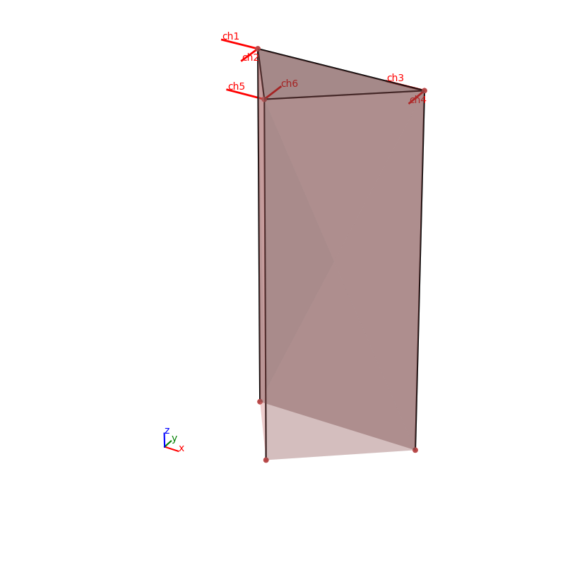
# (geometry2) with matplotlib
_, _ = Pali_ss.plot_geo2_mpl(scaleF=2)

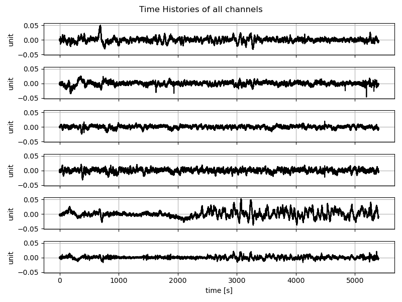
We can plot all the time histories of the channels calling the plot_data() method

# Plot the Time Histories
_, _ = Pali_ss.plot_data()

We can also get more info regarding the quality of the data for a specific channel calling the plot_ch_info() method

# Plot TH, PSD and KDE of the (selected) channels
_, _ = Pali_ss.plot_ch_info(ch_idx=[-1])

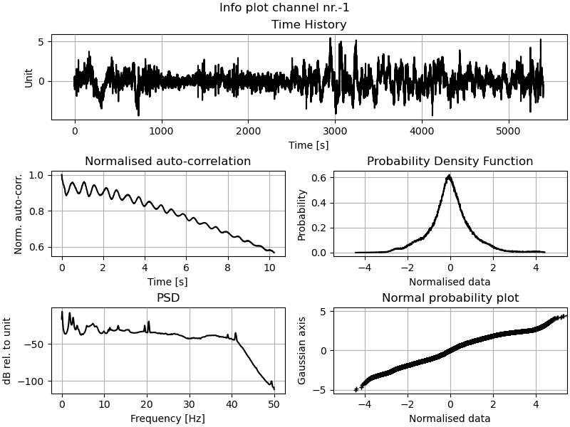
As we can see from the auto correlation there’s a low frequency component in the data.

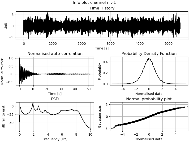
Other than the detrend_data() and decimate_data() methods there’s also a filter_data() method that can help us here.

# Detrend and decimate
#Pali_ss.detrend_data()
Pali_ss.filter_data(Wn=(0.1), order=8, btype="highpass")
Pali_ss.decimate_data(q=5)
_, _ = Pali_ss.plot_ch_info(ch_idx=[-1])

We need now to instantiate the algorithms that we want to run, e.g. FSDD and SSIcov. The algorithms must then be added to the setup class using the add_algorithms() method. Thereafter, the algorithms can be executed either individually using the run_by_name() method or collectively with run_all().

# Initialise the algorithms
fsdd = FSDD(name="FSDD", nxseg=1024, method_SD="cor")
ssicov = SSIcov(name="SSIcov", br=30, ordmax=30, calc_unc=True)
plscf = pLSCF(name="polymax",ordmax=30)

# Overwrite/update run parameters for an algorithm
fsdd.run_params = FSDD.RunParamCls(nxseg=2048, method_SD="per", pov=0.5)

# Add algorithms to the single setup class
Pali_ss.add_algorithms(ssicov, fsdd, plscf)

# Run all or run by name
Pali_ss.run_by_name("SSIcov")
Pali_ss.run_by_name("FSDD")
Pali_ss.run_by_name("polymax")
# Pali_ss.run_all()

# save dict of results
ssi_res = ssicov.result.model_dump()
fsdd_res = dict(fsdd.result)

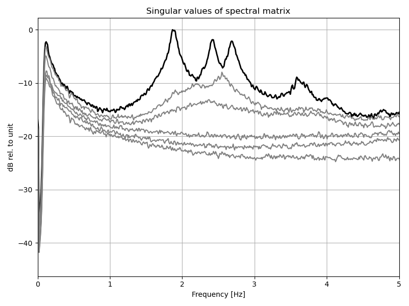
We can now plot some of the results:

# plot Singular values of PSD
_, _ = fsdd.plot_CMIF(freqlim=(1,4))

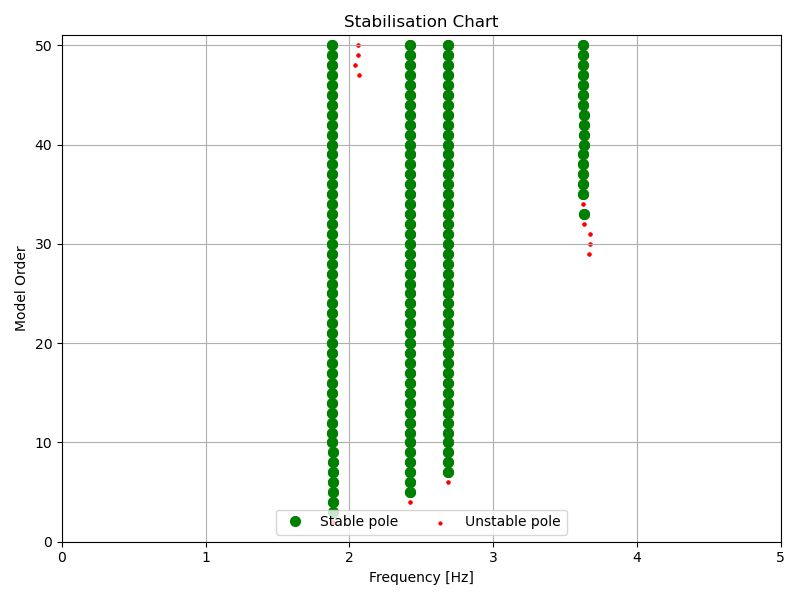
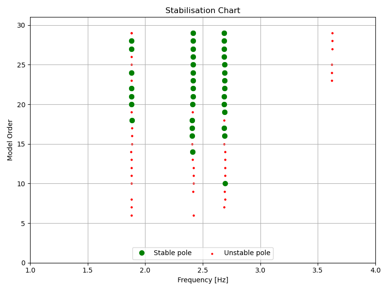
# plot Stabilisation chart for SSI
_, _ = ssicov.plot_stab(freqlim=(1,4), hide_poles=False)

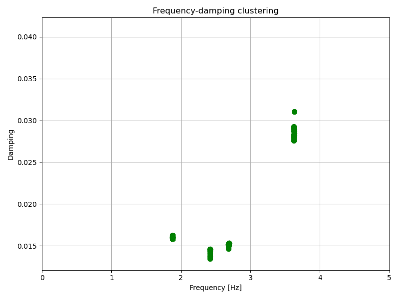
# plot frequecy-damping clusters for SSI
_, _ = ssicov.plot_freqvsdamp(freqlim=(1,4))

# plot Stabilisation chart for pLSCF
_, _ = plscf.plot_stab(freqlim=(1,4), hide_poles=False)

We are now ready to extract the modal properties of interest either from the interactive plots using the mpe_from_plot() method or using the mpe() method.

# Select modes to extract from plots
# Pali_ss.mpe_from_plot("SSIcov", freqlim=(1,4))

# or directly
Pali_ss.mpe("SSIcov", sel_freq=[1.88, 2.42, 2.68], order_in=20)

# update dict of results
ssi_res = dict(ssicov.result)

# Select modes to extract from plots
# Pali_ss.mpe_from_plot("FSDD", freqlim=(1,4), MAClim=0.95)

# or directly
Pali_ss.mpe("FSDD", sel_freq=[1.88, 2.42, 2.68], MAClim=0.95)

# update dict of results
fsdd_res = dict(fsdd.result)

We can compare the results from the two methods

ssicov.result.Fn

>>> array([1.88205042, 2.4211625 , 2.68851009])

fsdd.result.Fn

>>> array([1.8787832 , 2.42254302, 2.67381079])

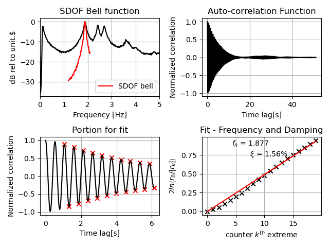
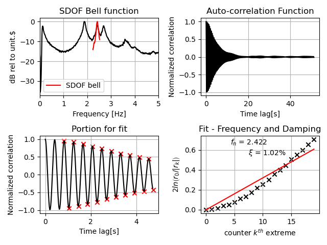
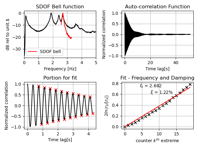
We can also plot some additional info regarding the estimates for the EFDD and FSDD algorithms

# plot additional info (goodness of fit) for EFDD or FSDD
_, _ = Pali_ss[fsdd.name].plot_EFDDfit(freqlim=(1,4))

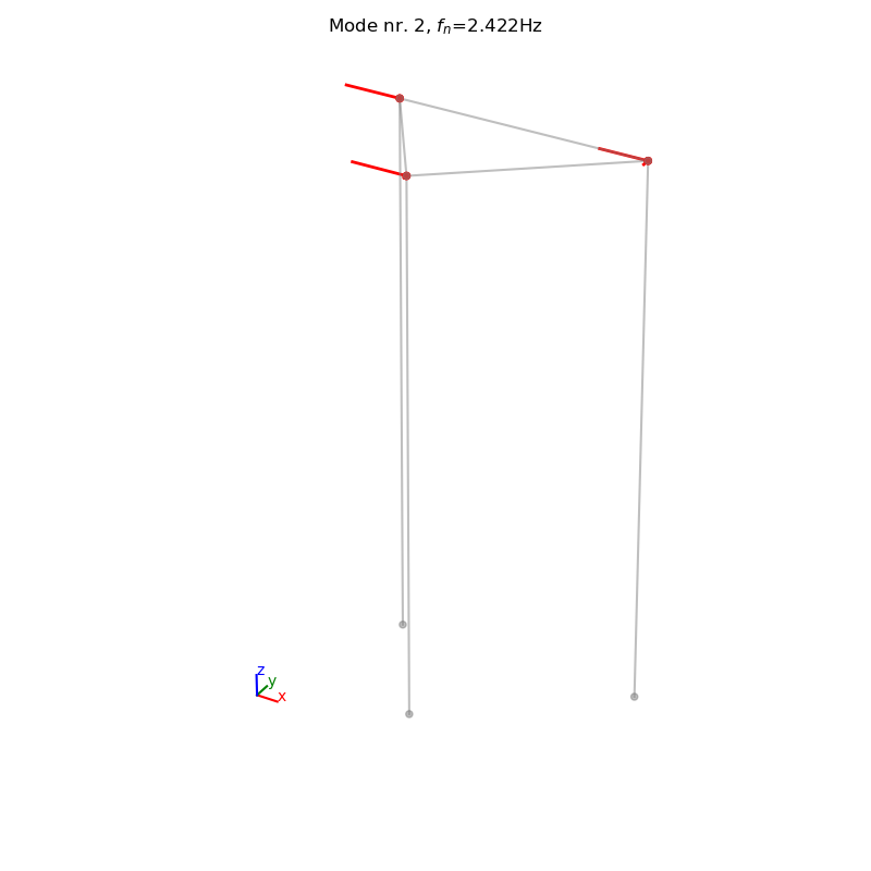
And finally we can plot and/or animate the mode shapes extracted from the analysis

# MODE SHAPES PLOT
# Plot mode 2 (geometry 1)
_, _ = Pali_ss.plot_mode_geo1(algo_res=fsdd.result, mode_nr=2, view="3D", scaleF=2)

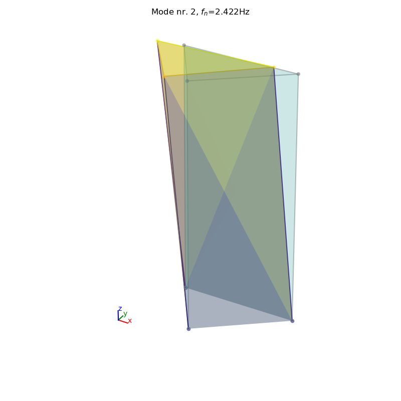
# Animate mode 1 (geometry 2)
_ = Pali_ss.anim_mode_geo2(
    algo_res=ssicov.result, mode_nr=1, scaleF=3)

It is also possible to save and load the results to a pickled file.

import os
import sys
import pathlib
# Add the directory we executed the script from to path:
sys.path.insert(0, os.path.realpath('__file__'))

from pyoma2.functions.gen import save_to_file, load_from_file

# Save setup
save_to_file(Pali_ss, pathlib.Path(r"./test.pkl"))

# Load setup
pali2: SingleSetup = load_from_file(pathlib.Path(r"./test.pkl"))

# plot from loded instance
_, _ = pali2.plot_mode_geo2_mpl(
    algo_res=fsdd.result, mode_nr=1, view="3D", scaleF=2)

# delete file
os.remove(pathlib.Path(r"./test.pkl"))

[APTF20]

Aloisio, A., Pasca, D., Tomasi, R., & Fragiacomo, M. (2020). Dynamic identification and model updating of an eight-storey CLT building. Engineering Structures, 213, 110593.