Example4 - Multisetup with Pre Global Estimation Re-scaling (PreGER) method

In this example, we’ll be working with a simulated dataset generated from a finite element model of a fictitious three-story, L-shaped building. This model was created using OpenSeesPy, and the corresponding Python script can be found here.

As always, first we import the necessary modules. All the files needed to run this example are available here.

import numpy as np
import pandas as pd
import matplotlib.pyplot as plt

from pyoma2.algorithms import SSIdat_MS
from pyoma2.setup import MultiSetup_PreGER
from pyoma2.support.utils.example_data import get_sample_data

For the preGER merging procedure, we adopt a strategy similar to that used for the single setup class. The first step involves instantiating the MultiSetup_PreGER class and passing the list of datasets, the lists of reference sensors, and their sampling frequency. Similarly to the single setup class, also for the MultiSetup_PreGER we have access to a wide set of tools to pre-process the data and get more information regarding its quality (e.g. decimate_data(), filter_data(), plot_ch_info() methods).

# import data files
set1 = np.load(get_sample_data(filename="set1.npy", folder="3SL")), allow_pickle=True)
set2 = np.load(get_sample_data(filename="set2.npy", folder="3SL")), allow_pickle=True)
set3 = np.load(get_sample_data(filename="set3.npy", folder="3SL")), allow_pickle=True)

# list of datasets and reference indices
data = [set1, set2, set3]
ref_ind = [[0, 1, 2], [0, 1, 2], [0, 1, 2]]

# Create multisetup
msp = MultiSetup_PreGER(fs=100, ref_ind=ref_ind, datasets=data)

# decimate data
msp.decimate_data(q=2)

# plot Time Histories of all channels for the selected datasets
msp.plot_data(data_idx=[2], nc=2)

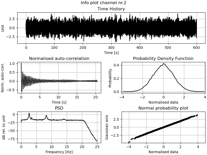
# Plot TH, PSD and KDE of the (selected) channels of the (selected) datasets
figs, axs = msp.plot_ch_info(data_idx=[1], ch_idx=[2])

Again if we want to be able to plot the mode shapes later, then we need to define the geometry of the structure.

# Geometry 1
_geo1 = get_sample_data(filename="Geo1.xlsx", folder="3SL")
# Geometry 2
_geo2 = get_sample_data(filename="Geo2.xlsx", folder="3SL")

# Define geometry1
msp.def_geo1_by_file(_geo1)
# Define geometry 2
msp.def_geo2_by_file(_geo2)

Now we need to instantiate the multi-setup versions of the algorithms we wish to execute, such as SSIdat.

# Initialise the algorithms
ssidat = SSIdat_MS(name="SSIdat", br=80, ordmax=80)

# Add algorithms to the class
msp.add_algorithms(ssidat)
msp.run_all()

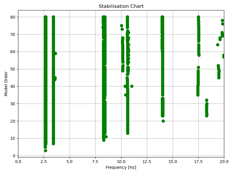
# Plot
ssidat.plot_stab(freqlim=20)

After the algorithms have been executed we can exctract the desired poles and plot the mode shapes.

# get modal parameters
msp.mpe(
      "SSIdat",
      sel_freq=[2.63, 2.69, 3.43, 8.29, 8.42, 10.62, 14.00, 14.09, 17.57],
      order_in=80)

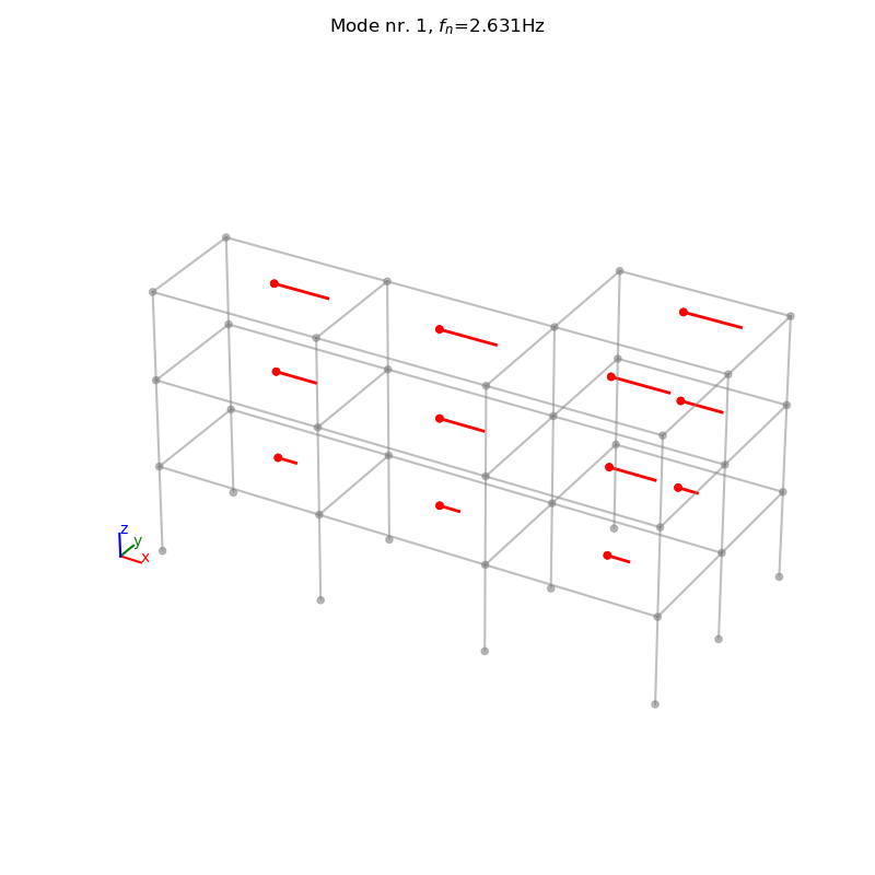
# plot mode shapes
msp.plot_mode_geo1(alg_res=SSIdat.result, mode_nr=1, view="3D", scaleF=2)
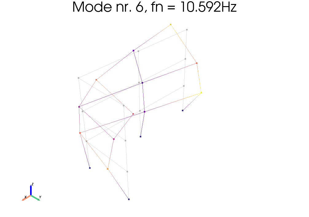
ssidat.plot_mode_geo2(geo2=msp.geo2, mode_nr=6, view="xy", scaleF=2)

ssidat.result.Fn

>>>   array([ 2.63102473,  2.69617968,  3.42605687,  8.27997956,  8.41882261,
            10.59171709, 13.96998337, 14.03397164, 17.49790384])