Example3 - Multisetup with Post Separate Estimation Re-scaling (PoSER) method

In this example, we’ll be working with a simulated dataset generated from a finite element model of a fictitious three-story, L-shaped building. This model was created using OpenSeesPy, and the corresponding Python script can be found here.

As always, first we import the necessary modules. All the files needed to run this example are available here.

import numpy as np
import pandas as pd
import matplotlib.pyplot as plt

from pyoma2.algorithms import SSIcov
from pyoma2.setup import MultiSetup_PoSER, SingleSetup
from pyoma2.support.utils.sample_data import get_sample_data

For the PoSER approach, after importing the necessary modules and loading the data, the next step is to create a separate instance of the single setup class for each available dataset.

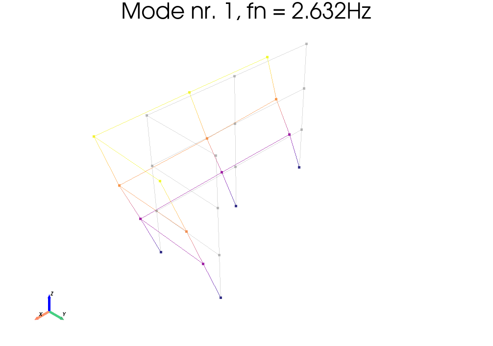
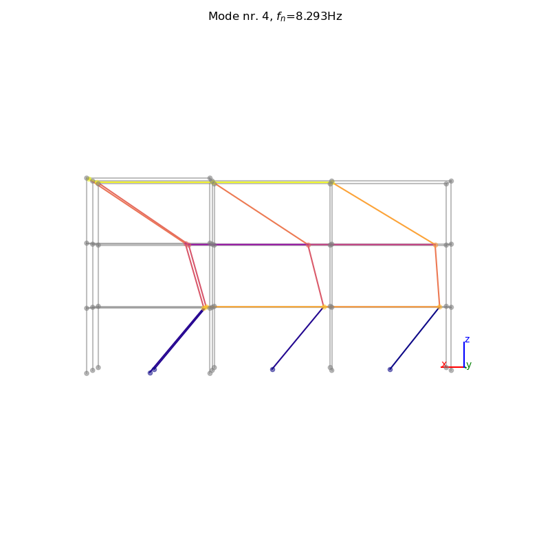
The exact natural frequencies of the system are: 2.63186, 2.69173, 3.43042, 8.29742, 8.42882, 10.6272, 14.0053, 14.093, 17.5741

# import data files
set1 = np.load(get_sample_data(filename="set1.npy", folder="3SL"), allow_pickle=True)
set2 = np.load(get_sample_data(filename="set2.npy", folder="3SL"), allow_pickle=True)
set3 = np.load(get_sample_data(filename="set3.npy", folder="3SL"), allow_pickle=True)

# create single setup
ss1 = SingleSetup(set1, fs=100)
ss2 = SingleSetup(set2, fs=100)
ss3 = SingleSetup(set3, fs=100)

# Detrend and decimate
ss1.decimate_data(q=2)
ss2.decimate_data(q=2)
ss3.decimate_data(q=2)

The process for obtaining the modal properties from each setup remains the same as described in the example for the single setup.

# Initialise the algorithms for setup 1
ssicov1 = SSIcov(name="SSIcov_s1", method="cov", br=50, ordmax=80)
# Add algorithms to the class
ss1.add_algorithms(ssicov1)
ss1.run_all()

# Initialise the algorithms for setup 2
ssicov2 = SSIcov(name="SSIcov_s2", method="cov", br=50, ordmax=80)
ss2.add_algorithms(ssicov2)
ss2.run_all()

# Initialise the algorithms for setup 3
ssicov3 = SSIcov(name="SSIcov_s3", method="cov", br=50, ordmax=80)
ss3.add_algorithms(ssicov3)
ss3.run_all()

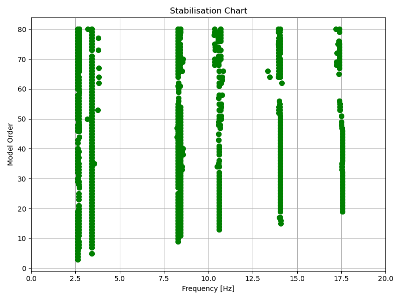
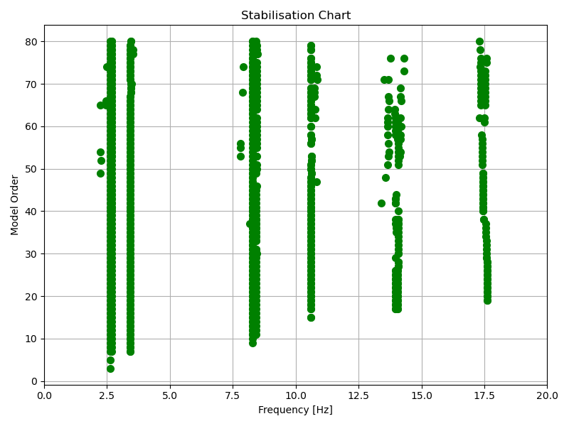
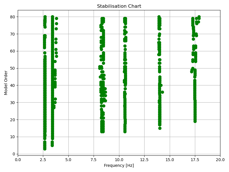
# Plot stabilisation chart
_, _ = ssicov1.plot_stab(freqlim=(1,20))
_, _ = ssicov2.plot_stab(freqlim=(1,20))
_, _ = ssicov3.plot_stab(freqlim=(1,20))

# Extract results
ss1.mpe(
    "SSIcov_s1",
    sel_freq=[2.63, 2.69, 3.43, 8.29, 8.42, 10.62, 14.00, 14.09, 17.57],
    order_in=50)
ss2.mpe(
    "SSIcov_s2",
    sel_freq=[2.63, 2.69, 3.43, 8.29, 8.42, 10.62, 14.00, 14.09, 17.57],
    order_in=40)
ss3.mpe(
    "SSIcov_s3",
    sel_freq=[2.63, 2.69, 3.43, 8.29, 8.42, 10.62, 14.00, 14.09, 17.57],
    order_in=40)

After analyzing all datasets, the MultiSetup_PoSER class can be instantiated by passing the processed single setup and the lists of reference indices. Subsequently, the merge_results() method is used to combine the results.

 # reference indices
 ref_ind = [[0, 1, 2], [0, 1, 2], [0, 1, 2]]
 # Creating Multi setup
 msp = MultiSetup_PoSER(ref_ind=ref_ind, single_setups=[ss1, ss2, ss3], names=["SSIcov"])

 # Merging results from single setups
 result = msp.merge_results()

 # dictionary of merged results
 res_ssicov = dict(result[SSIcov.__name__])
 result["SSIcov"].Fn

>>> array([ 2.63245926,  2.69030811,  3.4256547 ,  8.29328508,  8.42526299,
            10.60096486, 13.99307818, 14.09286017, 17.46931459])

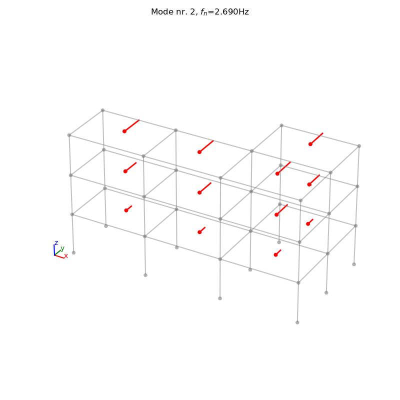
Once the class has been instantiated we can define the “global” geometry on it and then plot or animate the mode shapes

# Geometry 1
_geo1 = get_sample_data(filename="Geo1.xlsx", folder="3SL")
# Geometry 2
_geo2 = get_sample_data(filename="Geo2.xlsx", folder="3SL")

# Define geometry1
msp.def_geo1_by_file(_geo1)

# Define geometry 2
msp.def_geo2_by_file(_geo2)

# define results variable
algoRes = result[SSIcov.__name__]

# Plot mode 2 (geometry 1)
_, _ = msp.plot_mode_geo1(
      algo_res=algoRes, mode_nr=2, scaleF=2)

# Plot mode 1 (geometry 2, pyvista)
_ = msp.plot_mode_geo2(
      algo_res=algoRes, mode_nr=1, scaleF=3, notebook=True)

# Plot mode 4 (geometry 2, matplotlib)
_, _ = msp.plot_mode_geo2_mpl(
      algo_res=algoRes, mode_nr=4, view="xz", scaleF=3)

# Animate mode 5 (geometry 2, pyvista)
_ = msp.anim_mode_geo2(
      algo_res=algoRes, mode_nr=5, scaleF=3, notebook=True)

 algoRes.Fn

>>> array([ 2.63203919,  2.69132343,  3.4254799 ,  8.29357079,  8.42973383,
    10.60678491, 14.00410737, 14.08557463, 17.42890419])