Example1 - Getting started
In this first example we’ll take a look at a simple 5 degrees of freedom (DOF) system.
To access the data and the exact results of the system we can call the example_data() function in the submodule functions.gen
# import the function to generate the example dataset
from pyoma2.functions.gen import example_data

# assign the returned values
data, ground_truth = example_data()

# Print the exact results
np.set_printoptions(precision=3)
print(f"the natural frequencies are: {ground_truth[0]} \n")
print(f"the damping is: {ground_truth[2]} \n")
print("the (column-wise) mode shape matrix: \n"
f"{ground_truth[1]} \n")

>>> the natural frequencies are: [0.89  2.598 4.095 5.261 6.   ]
>>> the damping is: 0.02
>>> the (column-wise) mode shape matrix:
    [[ 0.285 -0.764  1.     0.919 -0.546]
    [ 0.546 -1.     0.285 -0.764  0.919]
    [ 0.764 -0.546 -0.919 -0.285 -1.   ]
    [ 0.919  0.285 -0.546  1.     0.764]
    [ 1.     0.919  0.764 -0.546 -0.285]]
Now we can instantiate the SingleSetup class, passing the dataset and the sampling frequency as arguments
from pyoma2.setup.single import SingleSetup

simp_5dof = SingleSetup(data, fs=600)
Since the maximum frequency is at approximately 6Hz, we can decimate the signal quite a bit.
To do this we can call the decimate_data() method
# Decimate the data
simp_5dof.decimate_data(q=30)
To analise the data we need to instanciate the desired algorithm to use with a name and the required arguments.
from pyoma2.algorithms.fdd import FDD
from pyoma2.algorithms.ssi import SSIdat

# Initialise the algorithms
fdd = FDD(name="FDD", nxseg=1024, method_SD="cor")
ssidat = SSIdat(name="SSIdat", br=30, ordmax=30)

# Add algorithms to the class
simp_5dof.add_algorithms(fdd, ssidat)

# run
simp_5dof.run_all()
We can now check the results
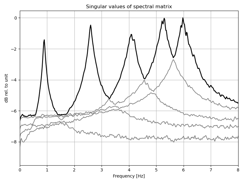
# plot singular values of the spectral density matrix
_, _ = fdd.plot_CMIF(freqlim=(0,8))
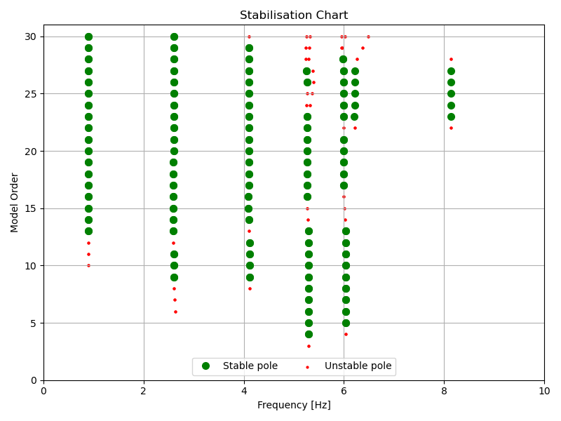
# plot the stabilisation diagram
_, _ = ssidat.plot_stab(freqlim=(0,10),hide_poles=False)
We can get the modal parameters with the help of an interactive plot calling the mpe_from_plot() method,
or we can get the results “manually” with the mpe() method.
# get the modal parameters with the interactive plot
# simp_ex.mpe_from_plot("SSIdat", freqlim=(0,10))

# or manually
simp_5dof.mpe("SSIdat", sel_freq=[0.89, 2.598, 4.095, 5.261, 6.], order_in="find_min")
Now we can now access all the results and compare them to the exact solution
# dict of results
ssidat_res = dict(ssidat.result)
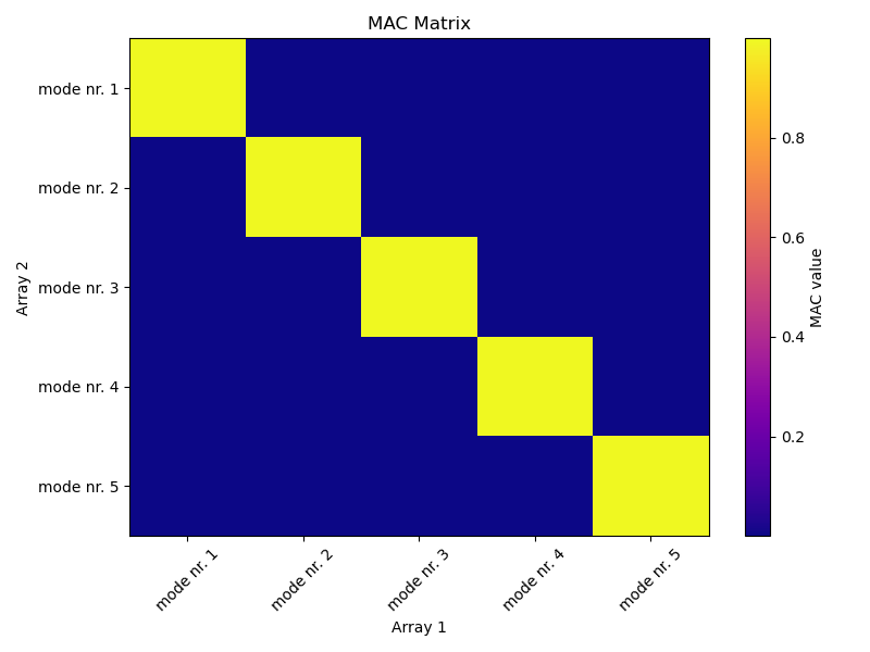
from pyoma2.functions.plot import plot_mac_matrix
# print the results
print(f"order out: {ssidat_res['order_out']} \n")
print(f"the natural frequencies are: {ssidat_res['Fn']} \n")
print(f"the dampings are: {ssidat_res['Xi']} \n")
print("the (column-wise) mode shape matrix:")
print(f"{ssidat_res['Phi'].real} \n")
_, _ = plot_mac_matrix(ssidat_res['Phi'].real, ground_truth[1])
>>> the natural frequencies are: [0.891 2.596 4.097 5.263 5.998]
>>> the dampings are: [0.022 0.019 0.025 0.019 0.019]
>>> the (column-wise) mode shape matrix:
[[ 0.312 0.773 1. 0.926 0.537]
[ 0.545 1. 0.279 -0.762 -0.912]
[ 0.774 0.541 -0.912 -0.283 1. ]
[ 0.985 -0.285 -0.534 1. -0.738]
[ 1. -0.942 0.749 -0.544 0.279]]